Sample Code of VMS stabilization in 2D Advection-Diffusion
written by M. Anguiano, L. Zhu and A. Masud (2019).
Reference:
Masud, A., & Khurram, R. A. (2004).
A multiscale/stabilized finite element method for the advection–diffusion equation.
Computer Methods in Applied Mechanics and Engineering, 193(21–22), 1997–2018.
https://doi.org/10.1016/j.cma.2003.12.047
Contents
Mesh generation
Mesh generation:  uniform Q4 element
nel_1D = 40; % Number of elements (1D)
nnode_1D = nel_1D + 1; % Number of nodes (1D)
x = linspace(0, nel_1D, nnode_1D);
% x_streched = 0.5 * (1.0 - cos(pi * x / nel_1D)); % 1D stretched
x_streched = x / nel_1D;
[Xcoord, Ycoord] = meshgrid(x_streched, x_streched); % Generate spatial grid

nnode = nnode_1D ^ 2; % Number of nodes (2D)
node_num = linspace(1, nnode, nnode); % Node numbering
node_num_mtx = reshape(node_num, [nnode_1D, nnode_1D]);
Gaussian Quadrature Rules

wght_1D = [5/9, 8/9, 5/9];
gp_loc_1D = [-sqrt(3/5), 0, sqrt(3/5)];
gp_2D = zeros(9, 3);
k = 0;
for i = 1:3
    for j = 1:3
        k = k + 1;
        gp_2D(k, :) = [gp_loc_1D(i), gp_loc_1D(j), wght_1D(i)*wght_1D(j)];
    end
end
Residual of the Variational Formulation
Advection-Diffusion Equation

u1 = zeros(nnode, 1);
u2 = zeros(nnode, 1);
p = zeros(nnode, 1);
R_global = zeros(nnode, 1);
K_global = zeros(nnode, nnode);
xl = zeros(2, 4);
for j = 1:nel_1D
    for i = 1:nel_1D
        xl(1,:) = [x_streched(i), x_streched(i+1), x_streched(i+1), x_streched(i)];
        xl(2,:) = [x_streched(j), x_streched(j), x_streched(j+1), x_streched(j+1)];
        node_el = [node_num_mtx(i,j), node_num_mtx(i+1,j), node_num_mtx(i+1,j+1), node_num_mtx(i,j+1)];

        % ==================== %
        % VMS stab. parameter tauHat
        tauHat = computeTauHat(xl,gp_2D);
        % ==================== %

        r_local = zeros(4, 1);
        k_local = zeros(4, 4);
        for l = 1 : 9
            % shape function and its derivatives at Gaussian point l
            [shg, jcb] = shp_bbl_Q4_adv(xl, gp_2D(l,1:2));
            % location of Gaussian point in physical coordinates
            x_GP = shg(3,1:4) * xl(1,:)';
            y_GP = shg(3,1:4) * xl(2,:)';

            %velocity vector
            amag = 1e6;
            thta = 67.5;
            avel(1) = amag*cosd(thta);
            avel(2) = amag*sind(thta);

            % Forcing function
            f_gp = 8 * pi^2 * sin(2*pi*x_GP) * sin(2*pi*y_GP); %Diffusion Test case
            f_gp = 0; %Advection-diffusion test cases

            % residual (forcing) at the Gaussian point
            r_gp = shg(3,1:4)' * f_gp;
            % stiffness matrix at the Gaussian point
            k_gp = shg(1,1:4)' * shg(1,1:4) + shg(2,1:4)' * shg(2,1:4) ...
                + shg(3,1:4)' * (avel * shg((1:2), 1:4));

            % ======================== %
            % VMS staibilization terms
            tau = shg(3,6)*tauHat;
            % tau = 0; % uncomment this line to revert back to Galerkin FEM,
            rstab_gp = tau * ((avel * shg(1:2, 1:4))' * f_gp );
            kstab_gp = tau * ((avel * shg(1:2, 1:4))' * (avel * shg((1:2), 1:4)));
            r_gp = r_gp + rstab_gp;
            k_gp = k_gp + kstab_gp;
            % ======================== %

            % consistent tangent* at the Gaussian point
            r_local = r_local + r_gp * jcb * gp_2D(l,3);
            k_local = k_local + k_gp * jcb * gp_2D(l,3);
        end
        R_global(node_el, 1) = R_global(node_el, 1) + r_local;
        K_global(node_el, node_el) = K_global(node_el, node_el) + k_local;
    end
end
Boundary Conditions
u_global = zeros(nnode, 1);
node_boun = [];
node_inte = [];
for j = 1:nnode_1D
    for i = 1:nnode_1D
        if i == 1 || j == 1  % || j == nnode_1D || i == nnode_1D
            node_boun = [node_boun, node_num_mtx(i,j)];

            % Non-zero dirichlet BC's
            if i == 1 || (i <= 0.2*nnode_1D && j == 1)
                u_global(node_num_mtx(i,j)) = 1;
            end

        else
            node_inte = [node_inte, node_num_mtx(i,j)];
        end
    end
end
Static Condensation
%u_global = zeros(nnode, 1);
u_global(node_inte) = K_global(node_inte, node_inte) \ (R_global(node_inte) - K_global(node_inte, node_boun) * u_global(node_boun));
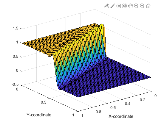
Visualization of the solution
surf(Xcoord , Ycoord , reshape(u_global, [nnode_1D, nnode_1D]));
zlim([-0.5, 1.5]);
xlabel('X-coordinate');
ylabel('Y-coordinate');

% Change viewing angle
[az,el] = view;
view(az+180,el);
Shape functions and bubble function and their derivatives for Q4 elements
Standard Q4 element
Quadratic bubble:  Advection bubble:
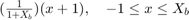
(cont'd): 
Here 
% input : xl(2,4)  nodal coordinates of the element
% input : gp(2)    location of Gaussion points
% input : xb(2)    location of internal virtual node
% output: shg(3,5) shape and bubble functions and their derivatives
% output: jcb      jacobian
function [shg, jcb] = shp_bbl_Q4_adv(xl, gp)
    shg = zeros(3, 5);
    x_el = xl(1,2) - xl(1,1); % x2 - x1
    y_el = xl(2,4) - xl(2,1); % y4 - y1
    jcb = x_el * y_el / 4; % affine elements only
    xi = gp(1); eta = gp(2);
    % shape functions
    shg(3,1) = 0.25 * (1 - xi) * (1 - eta);
    shg(3,2) = 0.25 * (1 + xi) * (1 - eta);
    shg(3,3) = 0.25 * (1 + xi) * (1 + eta);
    shg(3,4) = 0.25 * (1 - xi) * (1 + eta);
    % quadratic bubble
    shg(3,5) = (1 - xi^2) * (1 - eta^2);
    % advection bubble
    shg(3,6) = shg(3,1);    %for X_b = -0.99, Adv. bubble is approxed by N1
    % x derivative
    shg(1,1) = 0.25 * (-1 + eta);
    shg(1,2) = 0.25 * ( 1 - eta);
    shg(1,3) = 0.25 * ( 1 + eta);
    shg(1,4) = 0.25 * (-1 - eta);
    shg(1,5) = -2 * xi * (1 - eta^2);
    shg(1,6) = shg(1,1);
    % y derivative
    shg(2,1) = 0.25 * (-1 + xi);
    shg(2,2) = 0.25 * (-1 - xi);
    shg(2,3) = 0.25 * ( 1 + xi);
    shg(2,4) = 0.25 * ( 1 - xi);
    shg(2,5) = -2 * eta * (1 - xi^2);
    shg(2,6) = shg(2,1);
    % physical derivative
    shg(1,:) = shg(1,:) * 2 / x_el;
    shg(2,:) = shg(2,:) * 2 / y_el;
end
Stabilization Parameter
Standard Q4 element
This subroutine computes the stabilization parameter tau. This computation involves integration over the element domain, performed here via Gauss Quadrature of the same order as for the element subroutine.
% input : xl(2,4)  nodal coordinates of the element
% input : gp_2D    Gaussion points and weights
% output: tauHat   part of tau that is constant within the element
function [tauHat] = computeTauHat(xl, gp_2D)

    b2_int = 0;
    denom1_int = 0;
    denom2_int = 0;
    for l = 1 : 9
            % shape function and its derivatives at Gaussian point l
            [shg, jcb] = shp_bbl_Q4_adv(xl, gp_2D(l,1:2));
            % location of Gaussian point in physical coordinates
            x_GP = shg(3,1:4) * xl(1,:)';
            y_GP = shg(3,1:4) * xl(2,:)';

            % velocity vector
            amag = 1e6;
            thta = 67.5;
            avel(1) = amag*cosd(thta);
            avel(2) = amag*sind(thta);

            % Point Evalutions
            b2_gp = shg(3,6);
            denom1_gp = shg(1,6)' * shg(1,5) + shg(2,6)' * shg(2,5);
            denom2_gp = shg(3,6)' * (avel * shg(1:2,5));

            % Numerical Quadrature
            b2_int = b2_int + b2_gp * jcb * gp_2D(l,3);
            denom1_int = denom1_int + denom1_gp * jcb * gp_2D(l,3);
            denom2_int = denom2_int + denom2_gp * jcb * gp_2D(l,3);
    end

    tauHat = b2_int / (denom1_int + denom2_int);

end